研究动机与背景¶
生成式推荐与 Tokenizer 的瓶颈¶
生成式推荐(Generative Recommendation, GR)把召回 / 排序流水线统一成"对离散语义 ID 做 next-token prediction"。每个 item 被映射成一段离散 token 序列 $z_i = (z_i^{(1)}, \ldots, z_i^{(L)})$,序列模型自回归生成下一个 item 的 SID。这套范式让推荐质量的相当一部分负担转嫁给 tokenizer——如果 SID 的信息容量不够,生成器就只能在被劣化的目标上学习。
主流 tokenizer 沿两条线发展:parameter-free 方法(CID、GPTRec 用矩阵分解;SEATER、EAGER 用聚类)和 deep VQ 方法(TIGER 用 RQ-VAE 学层级离散 ID;LETTER 把协同信号注入 tokenizer;ETEGRec 做端到端联合优化;MMGRec、MACRec、MQL4GRec 引入多模态量化)。它们都共享一个未被审视的设计选择:所有 item 被分配相同长度的 SID——TIGER 的 4 层 RQ、LETTER 的 4 层、ETEGRec 的 4 层。这种均匀容量分配隐式假设所有 item 的信息需求相同。
Popularity-Length Paradox¶
作者在 Beauty / Sports / Toys / Yelp 四个数据集上做了一个 stratified evaluation:把测试样本按 ground-truth target item 的流行度划分为 Head(top 20%)/ Body(mid 60%)/ Tail(bottom 20%),分别评估 $L \in \{4, 6, 8, 10\}$ 下的 NDCG@10。结果(Figure 1)暴露出一个反直觉的结构性规律:
- Head 组:NDCG@10 随 $L$ 单调下降——$L=4$ 取得最佳,越长越差;
- Tail 组:NDCG@10 随 $L$ 单调上升——$L=10$ 取得最佳,越短越差;
- Body 组:在中间长度取得峰值;
- 整体最优固定长度只是一个对各群体都次优的折中。
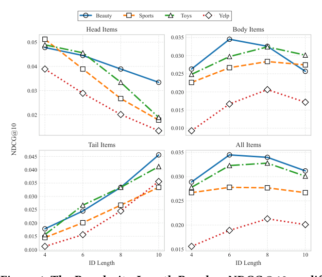
这个现象被命名为 Popularity-Length Paradox,是全文论证的起点。底层机制是信息充分性的不对称:popular item 在训练中频繁出现,积累了丰富的协同信号,短 SID 就足够判别;longer SID 会把推荐无关的细节强行编码进来,反而注入噪声。Tail item 交互稀疏,协同信号不可靠,必须依赖更细粒度的内容特征区分,需要更长的代码。
四个技术挑战¶
要把"按流行度自适应分配 SID 长度"做出来,必须同时解决四个互相耦合的难题:
- 长度选择缺乏理论依据——直觉告诉我们 popular 要短、tail 要长,但"短到多少、长到多少"需要一个可推导的最优 $L^*$。
- 欧氏残差量化的几何容量不够——标准 RQ 在 $\mathbb{R}^d$ 中,体积随半径多项式 $r^d$ 增长,要同时承载 4 层短 SID 和 10 层长 SID 的差异化容量,要么浅层冗余、要么深层失真。
- 长度决策本质上是离散的——选择 $L_i$ 是 hard truncation,无法直接对 $L_i$ 求梯度,端到端训练受阻。
- 变长 ID 的下游集成——同一 token 序列在变长设置下会出现 ID collision(如 (3,7) 与 (3,7,5) 共享前缀,可能撞到同一 item)、beam search 的 length bias(长 ID 因概率连乘累积更多负 log 项而被天然惩罚)、以及 hallucination(生成的序列不对应任何真实 item)。
VarLenRec 用四个互相耦合的组件分别回应这四个挑战:
- PIBA(Popularity-weighted Information Budget Allocation):把长度问题形式化为带正则的信息最大化,闭式证明最优长度按流行度的负幂次衰减;
- HARQ(Hyperbolic Adaptive Residual Quantization):把残差量化搬到 Poincaré 球,利用指数体积增长天然分层;
- Soft Length Controller:把离散长度决策松弛为每层保留概率的连续可微 gating,由 PIBA 推出的硬目标做正则;
- 下游集成:collision-resolving disambiguation token + Trie-constrained beam search + length-normalized rescoring。
四者通过 PIBA 紧密耦合——PIBA 既是 HARQ 几何选择的理论基础(容量应按 popularity 衰减),也是 Soft Length Controller 的监督信号(提供硬目标长度)。
核心方法¶
Problem Formulation¶
记 item 集合 $\mathcal{I} = \{i_1, \ldots, i_N\}$。Item $i$ 有内容特征 $\mathbf{x}_i \in \mathbb{R}^F$ 与流行度 $p_i$(归一化的训练交互频率,$\sum_i p_i = 1$)。目标是把每个 item 编码成变长 SID $\mathbf{z}_i = (z_i^{(1)}, \ldots, z_i^{(L_i)})$,其中 $z_i^{(l)} \in \{c_1^{(l)}, \ldots, c_M^{(l)}\}$ 索引第 $l$ 层 codebook,$L_i \in \{1, \ldots, K\}$ 是个体长度。
标准 fixed-length 方法的目标是最大互信息约束容量:
$$ \max_\theta I(X; Z) \quad \text{s.t.} \quad |Z| = L \tag{1} $$
这条目标把 $L$ 作为 hard 超参数,无法表达 popularity-dependent 容量需求。VarLenRec 重新定义为带编码成本正则的变长目标:
$$ \max_{L_i, \theta} I(X; Z_{1:L_i}) - \lambda \mathbb{E}[L_i] \tag{2} $$
其中 $Z_{1:L_i}$ 表示截断到长度 $L_i$ 的 ID,$\mathbb{E}[L_i]$ 是期望长度,$\lambda \gt 0$ 控制语义保真度与编码成本的权衡。
整体架构如下图:
Popularity-Weighted Information Budget Allocation(PIBA)¶
PIBA 把"item 需要多少容量"形式化为信息预算问题。每个 item 需要满足一个最低信息预算 $I_{\text{req}} \gt 0$ 才能被有效推荐,这个预算来自两条独立通道:
通道一:协同信号。交互越频繁,从 user-item co-occurrence 中能积累的信息越多。logarithmic gain 形式来自协同过滤的子模性结构(早期交互信息增益大、后续交互边际下降):
$$ I_{\text{collab}}(p_i) = \alpha \log(1 + \theta p_i) \tag{3} $$
$\alpha \gt 0$ 控制每个 log-popularity 单位的信息增益率,$\theta \gt 0$ 缩放基线交互频率。
通道二:语义 ID。按 rate-distortion theory 与 hierarchical quantization 的标准结论,第 $l$ 层量化贡献约 $\gamma / l$ bits(base capacity $\gamma \approx \log_2 M$ 由 codebook size 决定,深层贡献递减遵循 $1/l$ 谐波规律):
$$ I_{\text{semantic}}(L_i) = \gamma \sum_{l=1}^{L_i} \frac{1}{l} = \gamma H_{L_i} \approx \gamma \ln L_i \tag{4} $$
其中 $H_L$ 是 $L$-th harmonic number,渐近展开 $H_L \approx \ln L + \eta_{\text{EM}}$($\eta_{\text{EM}} \approx 0.5772$ 是 Euler-Mascheroni 常数)。
需要由 SID 补足的信息缺口是:
$$ G_i = I_{\text{req}} - \alpha \log(1 + \theta p_i) \tag{5} $$
Popular item 的 $G_i$ 小(短码即可填平),tail item 的 $G_i$ 大(需要长码)。
Theorem 1(Optimal Length Allocation). 在 Information Budget 框架下,最优 ID 长度 $L_i^*$ 满足 $\gamma \ln L_i^* \ge I_{\text{req}} - \alpha \log(1 + \theta p_i)$。对 $\theta p_i \gg 1$,使用 $\log(1 + \theta p_i) \approx \log \theta + \log p_i$ 近似:
$$ L_i^* = C \cdot p_i^{-\alpha / \gamma} \tag{6} $$
其中 $C = \exp((I_{\text{req}} - \alpha \log \theta) / \gamma) \gt 0$ 是与 popularity 无关的常数。最优长度按 popularity 的负幂次衰减——这就是 PIBA 的核心结论。
附录 A 给出完整证明:从 $I_{\text{semantic}}(L_i) \ge G_i$ 出发,等号取得时编码成本最小,求解 $L_i^*$ 即得 (6)。
离散化映射。$L_i^*$ 是连续值,必须离散为整数。VarLenRec 用 rank-based quantile mapping:按 popularity 降序排序 $r_i \in \{0, \ldots, N-1\}$($r_i = 0$ 最热门),归一化为 coldness $q_i = r_i / (N-1)$,再做温度变换 $\tilde{q}_i = q_i^\beta$($\beta \gt 0$ 对应 $\alpha / \gamma$)。最终离散映射:
$$ L_i = \mathrm{clip}\left(\mathrm{round}\left(1 + (K-1) \cdot \left(\frac{r_i}{N-1}\right)^\beta\right), 1, K\right) \tag{7} $$
保证 $p_a \gt p_b \Rightarrow L_a \le L_b$(单调性),且粒度由 $\beta$ 可控($\beta$ 大则长度对 popularity 更敏感)。
硬监督信号。从 (7) 得到的离散长度 $\hat{L}(p_i)$ 转成二元 mask $\mathbf{t}_i \in \{0,1\}^K$:
$$ t_i^{(l)} = \mathbb{1}\left[l \le \hat{L}(p_i)\right] \tag{8} $$
这条 mask 指示哪些层"应当被保留",作为 Soft Length Controller 的训练目标。整套机制称为 Popularity-weighted Information Budget Allocation (PIBA)。
HARQ:Hyperbolic Adaptive Residual Quantization¶
为什么需要双曲几何¶
标准向量量化在欧氏空间操作,多项式体积增长 $V_{\text{Eucl}}(r) \to r^d$。但 item 语义往往具备层级树状结构(大类→子类→细类),树的叶子数随深度呈指数增长——欧氏球只能提供多项式容量,结构上不匹配。
双曲空间提供指数体积增长。在 Poincaré ball $\mathbb{D}_c^d = \{\mathbf{x} \in \mathbb{R}^d : \|\mathbf{x}\| \lt 1/\sqrt{c}\}$ (curvature $-c$,$c \gt 0$) 中:
$$ V_{\text{Hyp}}(r) \sim \sinh^{d-1}(\sqrt{c} r) \approx e^{(d-1)\sqrt{c} r} $$
Theorem 2(Hyperbolic Representational Capacity). 在 Poincaré ball 中,距离原点 $r$ 时可区分区域数 $N(r) = \Theta(e^{(d-1)\sqrt{c}(r-\delta/2)})$(附录 D.1 证明)。这意味着 item 表示沿径向距离 $r$ 增长时,判别力指数级扩张——天然支持变长长度分配的需求。
Hyperbolic Embedding Space¶
VarLenRec 把 hyperbolic encoder 设计为先在欧氏空间编码再投影到 manifold:
$$ \mathbf{h}_i = \mathrm{MLP}_{\text{enc}}(\mathbf{x}_i) \in \mathbb{R}^d, \quad \mathbf{z}_i^{(0)} = \exp_0^c(\mathbf{h}_i) \in \mathbb{D}_c^d $$
Encoder 学到把 popular item 放在 origin 附近(紧凑),把 tail item 推向 boundary(按指数体积扩张取得 fine-grained 区分能力)。
Mobius addition(双曲加法):
$$ \mathbf{x} \oplus_c \mathbf{y} = \frac{(1 + 2c \langle \mathbf{x}, \mathbf{y} \rangle + c\|\mathbf{y}\|^2)\mathbf{x} + (1 - c\|\mathbf{x}\|^2)\mathbf{y}}{1 + 2c \langle \mathbf{x}, \mathbf{y} \rangle + c^2 \|\mathbf{x}\|^2 \|\mathbf{y}\|^2} \tag{9} $$
双曲距离:
$$ d_{\mathbb{D}}(\mathbf{x}, \mathbf{y}) = \frac{2}{\sqrt{c}} \mathrm{arctanh}(\sqrt{c} \| -\mathbf{x} \oplus_c \mathbf{y}\|) \tag{10} $$
指数映射(tangent → manifold):
$$ \exp_0^c(\mathbf{v}) = \tanh(\sqrt{c}\|\mathbf{v}\|) \frac{\mathbf{v}}{\sqrt{c}\|\mathbf{v}\|} \tag{11} $$
对数映射(manifold → tangent):
$$ \log_0^c(\mathbf{x}) = \frac{1}{\sqrt{c}} \mathrm{arctanh}(\sqrt{c}\|\mathbf{x}\|) \frac{\mathbf{x}}{\|\mathbf{x}\|} \tag{12} $$
Hyperbolic Residual Quantization¶
每层 $l$ 维护 codebook $\mathcal{E}^{(l)} = \{\mathbf{e}_1^{(l)}, \ldots, \mathbf{e}_M^{(l)}\}$(码字在 $\mathbb{D}_c^d$ 上)。初始化 $\mathbf{r}_i^{(0)} = \mathbf{z}_i^{(0)}$,每层选最近码字:
$$ z_i^{(l)} = \arg\min_{j \in \{1, \ldots, M\}} d_{\mathbb{D}}(\mathbf{r}_i^{(l-1)}, \mathbf{e}_j^{(l)}) \tag{13} $$
通过 Mobius 加上负码字算残差:
$$ \mathbf{r}_i^{(l)} = (-\mathbf{e}_{z_i^{(l)}}^{(l)}) \oplus_c \mathbf{r}_i^{(l-1)} \tag{14} $$
Soft Length Controller¶
为了让长度决策可微,每层引入一个 lightweight gate network 预测"保留概率" $\alpha_i^{(l)}$。具体地,在第 $l$ 层,把残差 $\mathbf{r}_i^{(l)}$ 与选中的码字 $\mathbf{e}_{z_i^{(l)}}^{(l)}$ 都用 $\log_0^c$ 投影到 tangent space,concat 后送入 gate MLP:
$$ \alpha_i^{(l)} = \sigma\left(\mathrm{MLP}_{\text{gate}}([\log_0^c(\mathbf{r}_i^{(l-1)}); \log_0^c(\mathbf{e}_{z_i^{(l)}}^{(l)})])\right) \tag{15} $$
$\sigma$ 是 sigmoid。关键设计:gate 同时看到当前残差与刚选中的码字——如果残差已被早期层充分捕获,gate 自动学到提早终止;否则继续往深层走。
为强制 prefix 约束(保留第 $l$ 层必须保留所有前序层),定义累积 mask:
$$ m_i^{(l)} = \prod_{j=1}^{l} \alpha_i^{(j)} \tag{16} $$
这些连续 mask 训练时支持端到端可微,推理时通过阈值离散化:选 $L_i = \arg\max_l \{m_i^{(l)} \ge \tau\}$($\tau \in (0,1)$,论文设 $\tau = 0.5$)。等价地,保留层 $l$ 当且仅当 $\alpha_i^{(l)} \ge \tau$。
Hyperbolic Decoder¶
按软 mask 重构 item 表示:从 $\tilde{\mathbf{z}}_i^{(0)} = \mathbf{0}$ 开始:
$$ \tilde{\mathbf{z}}_i^{(l)} = \tilde{\mathbf{z}}_i^{(l-1)} \oplus_c \mathrm{Scale}_c(m_i^{(l)}, \mathbf{e}_{z_i^{(l)}}^{(l)}) \tag{17} $$
其中 $\mathrm{Scale}_c(s, \mathbf{v}) = \exp_0^c(s \cdot \log_0^c(\mathbf{v}))$ 是双曲标量乘。$\tilde{\mathbf{z}}_i = \tilde{\mathbf{z}}_i^{(K)}$ 经对数映射回欧氏并经 decoder MLP 得到重构特征 $\hat{\mathbf{x}}_i$。
Training Objectives¶
四项 loss 协同优化:
(i) Reconstruction loss:
$$ \mathcal{L}_{\text{recon}} = \|\mathbf{x}_i - \hat{\mathbf{x}}_i\|^2 $$
(ii) Quantization loss(双曲距离 + 码字 commitment):
$$ \mathcal{L}_{\text{quant}} = \sum_{l=1}^{K} \left[d_{\mathbb{D}}(\mathrm{sg}[\mathbf{r}_i^{(l-1)}], \hat{\mathbf{e}}_i^{(l)})^2 + \beta \cdot d_{\mathbb{D}}(\mathbf{r}_i^{(l-1)}, \mathrm{sg}[\hat{\mathbf{e}}_i^{(l)}])^2\right] \tag{18} $$
其中 $\hat{\mathbf{e}}_i^{(l)} = \mathbf{e}_{z_i^{(l)}}^{(l)}$,$\mathrm{sg}[\cdot]$ 是 stop-gradient,$\beta$ 是 commitment 系数。第一项把码字拉向残差,第二项把残差表示推向选中的码字。
(iii) Length cost loss(抑制 over-deep):
$$ \mathcal{L}_{\text{cost}} = \sum_{l=1}^{K} m_i^{(l)} $$
(iv) Length alignment loss(与 PIBA 硬目标对齐):用二元交叉熵把每层 cumulative mask $m_i^{(l)}$ 推向 PIBA 推出的硬目标 $t_i^{(l)}$:
$$ \mathcal{L}_{\text{len}} = -\sum_{l=1}^{K} \left[t_i^{(l)} \log m_i^{(l)} + (1 - t_i^{(l)}) \log(1 - m_i^{(l)})\right] \tag{19} $$
这条 loss 是把信息论先验注入网络的关键——它鼓励 popular item 准确激活 $\hat{L}(p_i)$ 层后停止,tail item 启用更深层。
整体目标:
$$ \mathcal{L} = \mathcal{L}_{\text{recon}} + \mathcal{L}_{\text{quant}} + \lambda_{\text{cost}} \mathcal{L}_{\text{cost}} + \lambda_{\text{len}} \mathcal{L}_{\text{len}} \tag{20} $$
用 Riemannian Adam(附录 E)优化,把欧氏梯度按共形因子 $\lambda_{\mathbf{w}}^{-2}$ 调整后通过 exponential map 投影回 manifold;并对码字向量加 safety margin $\epsilon = 10^{-5}$ 防止飞出 Poincaré ball boundary。
Variable-Length ID Integration(下游集成)¶
训完 HARQ tokenizer 后,把变长 SID 喂给 Transformer-based 生成器(VarLenRec 用 T5 backbone)做 token-by-token autoregressive next-item prediction,遇到 EOS 终止。但变长 SID 在生成阶段会带来三个新麻烦:
Challenge 1:ID Collision¶
在固定长度场景,撞 SID 时可通过附加 disambiguation token 解决(不影响其他 item)。变长场景下,从原 codebook $\{1, \ldots, M\}$ 拿一个 token 附到短 ID 后面,可能与一个本来更长的 ID 撞车(例如 $(3, 7, 5)$ 已存在,把 5 加到 $(3, 7)$ 上就坍塌了)。
解法:开辟一个不相交的辅助 codebook $\{M+1, \ldots, 2M\}$,专门用于 post-hoc disambiguation。当两个 item 撞到 $(3, 7)$ 时,从这段附加 token 中取唯一标识,得 $(3, 7, M+1)$、$(3, 7, M+2)$。这条设计保证 disambiguation 操作不会污染语义量化层的训练。
Challenge 2:Hallucination¶
变长 ID 让生成空间膨胀,beam search 可能产生不对应任何真实 item 的序列。解法:构造前缀树 $\mathcal{T}$,包含所有 collision-resolved 真实 ID。每个 decoding step 用 Trie-constrained beam search,只探索 $\mathcal{T}$ 中合法的子结点。
Challenge 3:Length Bias¶
beam search 用标准 log-probability 评分 $\log P(\hat{\mathbf{z}} \mid \mathbf{z}_{S_u})$,长度 $L$ 的 ID 累积约 $L$ 个负 log 项——天然偏向短 ID。这条 artificial length penalty 会反向破坏 PIBA 的长度分配(让长 ID 总是被压下去)。
解法:采用 [4] 提出的 rescoring 范式。Trie-constrained beam search 用标准 log-prob 走完,收集所有 partial decoded candidate。beam search 完成后,用 odds ratio 公式对所有候选 $\hat{\mathbf{z}}$ 重新打分:
$$ s(\hat{\mathbf{z}}) = \max\left(0, \log\left(\frac{P(\hat{\mathbf{z}} \mid \mathbf{z}_{S_u})}{1 - P(\hat{\mathbf{z}} \mid \mathbf{z}_{S_u})} \cdot \frac{1 - P(\hat{\mathbf{z}})}{P(\hat{\mathbf{z}})}\right)\right) \tag{21} $$
$P(\hat{\mathbf{z}})$ 是 ID prefix 的归一化经验频率。这个 odds ratio 形式同时奖励"高条件概率"与"低边缘频率"(防止 popular 共同前缀垄断),并实现长度无关的最终排序。
实验设置¶
数据集¶
四个公开数据集,按 5-core 过滤后 leave-one-out 切分(最后一项 test、倒数第二验证、其余训练):
| Dataset | 用途 |
|---|---|
| Amazon Beauty | 化妆品类目 |
| Amazon Sports and Outdoors | 运动户外 |
| Amazon Toys and Games | 玩具游戏 |
| Yelp | 商家点评 |
Baselines¶
三大类共 13 个:
- 传统 sequential:HGN、GRU4Rec、BERT4Rec、SASRec、FMLP、$S^3$-Rec、HSTU
- Semantic ID-based:TIGER、LC-Rec、ETEGRec
- Enhanced GR:LETTER 应用于 TIGER 与 LC-Rec(即 LETTER-TIGER、LETTER-LCRec)
VarLenRec 集成两个 backbone:VarLenRec-TIGER 与 VarLenRec-LCRec。
评估指标¶
Recall@K 与 NDCG@K,$K \in \{5, 10\}$。全集 ranking(不做 negative sampling)。
实现细节¶
所有生成式方法共用 Sentence-T5 做 item 文本嵌入。Codebook size $M = 256$,最大 SID 长度 $K = 10$。双曲曲率 $c = 1.0$。超参 $\beta$、$\lambda_{\text{cost}}$、$\lambda_{\text{len}}$ 在 Appendix B 分析(验证集调),inference 时 $\tau = 0.5$。HARQ tokenizer 训练用 Riemannian Adam(lr 1e-4,bs 256);生成器(T5)用标准 Adam(lr 1e-4,bs 256);beam search beam size 30;NVIDIA A800 GPU。
主要实验结果(RQ1)¶
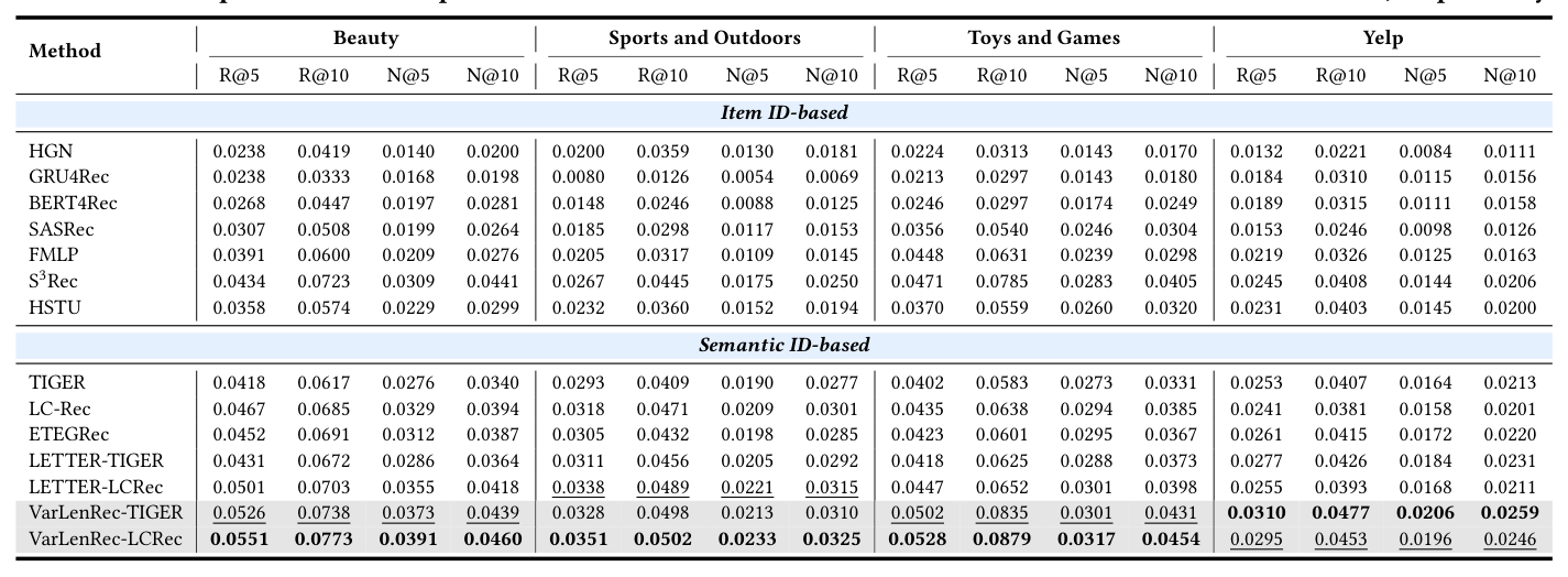
| Method | Beauty R@5 | R@10 | N@5 | N@10 | Sports R@5 | R@10 | N@5 | N@10 | Toys R@5 | R@10 | N@5 | N@10 | Yelp R@5 | R@10 | N@5 | N@10 |
|---|---|---|---|---|---|---|---|---|---|---|---|---|---|---|---|---|
| HGN | 0.0238 | 0.0419 | 0.0140 | 0.0200 | 0.0200 | 0.0359 | 0.0130 | 0.0181 | 0.0224 | 0.0313 | 0.0143 | 0.0170 | 0.0132 | 0.0221 | 0.0084 | 0.0111 |
| GRU4Rec | 0.0238 | 0.0333 | 0.0168 | 0.0198 | 0.0080 | 0.0126 | 0.0054 | 0.0069 | 0.0213 | 0.0297 | 0.0143 | 0.0156 | 0.0184 | 0.0310 | 0.0115 | 0.0156 |
| BERT4Rec | 0.0268 | 0.0447 | 0.0197 | 0.0281 | 0.0148 | 0.0246 | 0.0088 | 0.0125 | 0.0246 | 0.0297 | 0.0174 | 0.0249 | 0.0189 | 0.0315 | 0.0111 | 0.0158 |
| SASRec | 0.0307 | 0.0508 | 0.0199 | 0.0264 | 0.0185 | 0.0298 | 0.0117 | 0.0153 | 0.0356 | 0.0540 | 0.0246 | 0.0304 | 0.0153 | 0.0246 | 0.0099 | 0.0126 |
| FMLP | 0.0391 | 0.0600 | 0.0209 | 0.0276 | 0.0205 | 0.0317 | 0.0109 | 0.0145 | 0.0448 | 0.0631 | 0.0239 | 0.0298 | 0.0219 | 0.0326 | 0.0125 | 0.0163 |
| $S^3$-Rec | 0.0434 | 0.0723 | 0.0309 | 0.0441 | 0.0267 | 0.0445 | 0.0175 | 0.0250 | 0.0471 | 0.0785 | 0.0283 | 0.0405 | 0.0245 | 0.0408 | 0.0144 | 0.0206 |
| HSTU | 0.0358 | 0.0574 | 0.0229 | 0.0299 | 0.0232 | 0.0360 | 0.0152 | 0.0194 | 0.0370 | 0.0576 | 0.0260 | 0.0320 | 0.0231 | 0.0403 | 0.0145 | 0.0200 |
| TIGER | 0.0418 | 0.0617 | 0.0276 | 0.0340 | 0.0293 | 0.0409 | 0.0190 | 0.0277 | 0.0402 | 0.0583 | 0.0273 | 0.0331 | 0.0253 | 0.0407 | 0.0164 | 0.0213 |
| LC-Rec | 0.0467 | 0.0685 | 0.0329 | 0.0394 | 0.0318 | 0.0471 | 0.0209 | 0.0301 | 0.0435 | 0.0638 | 0.0294 | 0.0385 | 0.0241 | 0.0381 | 0.0158 | 0.0201 |
| ETEGRec | 0.0452 | 0.0691 | 0.0312 | 0.0387 | 0.0305 | 0.0432 | 0.0198 | 0.0285 | 0.0423 | 0.0601 | 0.0295 | 0.0367 | 0.0261 | 0.0415 | 0.0172 | 0.0220 |
| LETTER-TIGER | 0.0431 | 0.0672 | 0.0286 | 0.0364 | 0.0311 | 0.0456 | 0.0205 | 0.0292 | 0.0418 | 0.0625 | 0.0290 | 0.0367 | 0.0258 | 0.0420 | 0.0184 | 0.0211 |
| LETTER-LCRec | 0.0501 | 0.0703 | 0.0355 | 0.0418 | 0.0338 | 0.0489 | 0.0221 | 0.0315 | 0.0447 | 0.0652 | 0.0301 | 0.0398 | 0.0255 | 0.0393 | 0.0166 | 0.0211 |
| VarLenRec-TIGER | 0.0526 | 0.0738 | 0.0373 | 0.0439 | 0.0328 | 0.0498 | 0.0213 | 0.0310 | 0.0502 | 0.0835 | 0.0301 | 0.0431 | 0.0310 | 0.0477 | 0.0206 | 0.0259 |
| VarLenRec-LCRec | 0.0551 | 0.0773 | 0.0391 | 0.0460 | 0.0351 | 0.0502 | 0.0233 | 0.0325 | 0.0528 | 0.0879 | 0.0317 | 0.0454 | 0.0295 | 0.0453 | 0.0196 | 0.0246 |
逐项解读:
- VarLenRec-TIGER 全面超越 TIGER:以 Beauty 为例,R@10 从 0.0617 → 0.0738(+19.6%),N@10 从 0.0340 → 0.0439(+29.1%),表明变长机制对 fixed-length GR backbone 是正交的增益。
- VarLenRec-LCRec 全面超越 LCRec:Beauty R@10 0.0685 → 0.0773(+12.8%),证明对 fine-tuned LLM-based GR 同样有效。
- 超越 enhanced baseline LETTER:在 LETTER 已经把协同信号注入 tokenizer 后,VarLenRec 仍能再叠加变长机制的额外增益——两者正交,可以叠加。
- 超越所有传统 sequential 包括 HSTU。S³-Rec 是最强的非生成基线,VarLenRec-LCRec 在 Beauty R@10 上仍领先 6.9%(0.0773 vs 0.0723)。
- 数据集差异:Toys 上 R@10 增益最大(0.0835 / 0.0879 vs TIGER 0.0583,相对 +43% / +51%),与该数据集的 item 类别多样性高、Tail 比例大的特点一致——adaptive 容量分配空间最大。Yelp 上 VarLenRec-TIGER 取得最佳(其商家类目语义异质性最高)。
消融研究(RQ2)¶
| Variant | Beauty R@10 | Beauty N@10 | Toys R@10 | Toys N@10 |
|---|---|---|---|---|
| VarLenRec-TIGER(full) | 0.0738 | 0.0439 | 0.0835 | 0.0431 |
| Training Objective Ablation | ||||
| w/o $\mathcal{L}_{\text{cost}}$ | 0.0701 | 0.0415 | 0.0789 | 0.0403 |
| Fixed Length Baselines(w/o $\mathcal{L}_{\text{cost}}$ 与 $\mathcal{L}_{\text{len}}$) | ||||
| Fixed Length = 4 | 0.0652 | 0.0378 | 0.0623 | 0.0352 |
| Fixed Length = 6 | 0.0671 | 0.0392 | 0.0658 | 0.0371 |
| Fixed Length = 8 | 0.0659 | 0.0385 | 0.0641 | 0.0362 |
| Fixed Length = 10 | 0.0637 | 0.0342 | 0.0583 | 0.0337 |
| Length Prediction Ablation | ||||
| w/ Direct PIBA Assignment | 0.0716 | 0.0426 | 0.0777 | 0.0401 |
| Embedding Space Ablation | ||||
| w/ Euclidean Space | 0.0692 | 0.0408 | 0.0773 | 0.0395 |
| Inference Integration Ablation | ||||
| w/o Inference Strategies | 0.0681 | 0.0398 | 0.0765 | 0.0387 |
逐项分析:
- Training objective:去掉 $\mathcal{L}_{\text{cost}}$ 导致 Beauty R@10 掉 5.0%——模型会任意长 ID 浪费 sparsity 正则。
- Fixed length 全面输:$L=6$ 是固定长度的甜区,但仍比 adaptive 低 9.1%/21%(Beauty/Toys R@10)。没有任何固定长度能并列——证明 Popularity-Length Paradox 不是 hyperparameter 选择问题,是结构性问题。$L=10$ 比 $L=6$ 还差,符合"head item 在过长 ID 上反退化"的论文论断。
- Length prediction:用 PIBA 硬目标直接分配(不走 Soft Length Controller)相比 full version 在 Beauty/Toys 上分别低 3.0%/7.0%——content-aware 适应对语义复杂 item 尤为关键,纯 popularity-driven 不够。
- Embedding space:把 Poincaré ball 换成欧氏 RQ-VAE,Beauty R@10 掉 6.2%、Toys 掉 7.4%——验证 hyperbolic geometry 的指数体积更适合层级 item 语义。
- Inference integration:去掉 collision resolution + Trie-constrained + length-normalized 三件套,Beauty R@10 掉 7.7%、Toys 掉 8.4%。三者协同保证变长 ID 能被有效检索。
效率分析(RQ3)¶
| Method | Beauty Train | Beauty Test | Sports Train | Sports Test | Toys Train | Toys Test | Yelp Train | Yelp Test |
|---|---|---|---|---|---|---|---|---|
| TIGER | 37.1 | 87.2 | 45.3 | 106.8 | 35.8 | 82.4 | 52.6 | 124.3 |
| LETTER-TIGER | 40.4 | 92.4 | 49.2 | 113.5 | 38.9 | 87.6 | 57.1 | 131.8 |
| ETEGRec | 48.6 | 107.3 | 58.7 | 132.4 | 46.3 | 101.2 | 68.4 | 152.9 |
| VarLenRec-TIGER | 32.2 | 72.3 | 39.1 | 88.7 | 31.0 | 68.5 | 45.8 | 103.2 |
(数值:秒/epoch)
VarLenRec 在效率上同样领先——比 TIGER 训练快 15.8%、测试快 19.3%。原因是 popular item 用短 ID(实际 token 处理量减少),inference 时 early termination 进一步省 decoding step。变长不仅提升精度,还减小计算。这是反直觉的——添加复杂度通常带来开销,但这里 adaptive length 自身就是 sparsity 机制。
语义 ID 质量分析¶
Collision rate¶
附录 C.1 显示 collision rate 从 12.7%(fixed-length RQ-VAE baseline TIGER L=10)降到 3.2%(VarLenRec with HARQ),降幅 ~74%。Euclidean-space 变体(无 HARQ)只能降到中间水平(5-12%)——hyperbolic geometry 与 variable-length 两者协同才能把 collision 降到很低水平。
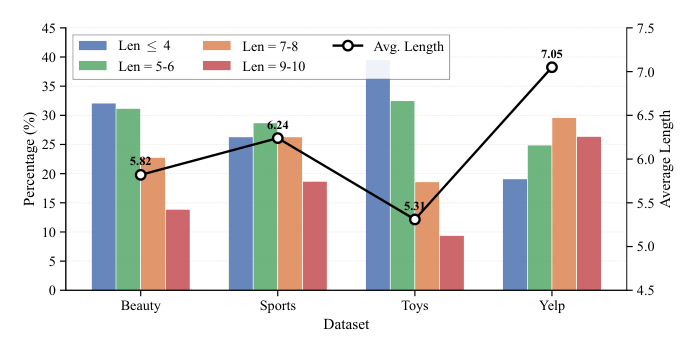
Length distribution¶
学到的长度分布因数据集而异:
- Yelp(商家点评,类目最异质):平均长度 7.05,56.0% item 长度 ≥ 7;
- Toys(标准化产品类目):平均长度 5.31,39.5% 长度 ≤ 4;
- Beauty / Sports 介于中间,分布近似 bell-shaped 集中在 5-6。
这说明 VarLenRec 把数据集本身的语义异质性学进了长度分布——结构化数据集偏短 ID、异质数据集偏长 ID。
Performance scaling by popularity¶
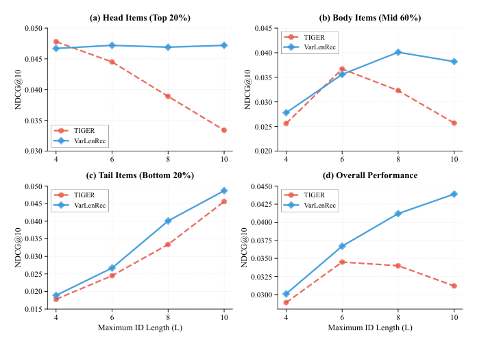
在 Beauty 上做 fine-grained 分析(按 max ID length L 与 popularity tier 切片,与 TIGER 对比):
- Head(top 20%):TIGER 在 $L=4$ 达峰值 0.0478,$L=10$ 退化 30.1%;VarLenRec 几乎不退化——验证了 head item 不需要长 ID,VarLenRec 不会强加冗余容量。
- Body(mid 60%):单调改进。
- Tail(bottom 20%):TIGER 从 $L=4$ 到 $L=10$ 改进 156.2%;VarLenRec 改进 +6.8% 还能稳定——更重要的是它不需要手工选 L,每个 item 自适应。
- Overall:单调改进,与 Theorem 1 的"length should adapt to information requirement"一致。
跨群体改进:head +41.3%、body +48.6%、tail +6.8%。Head 增益最大乍看反直觉,实际是因为之前 head item 被强行喂过长 ID 注入噪声,VarLenRec 把它们恢复到短 ID 后真正解放——而 tail item 之前已经在 long ID 设置下尽力,可改进空间相对小。
超参数敏感性(附录 B)¶
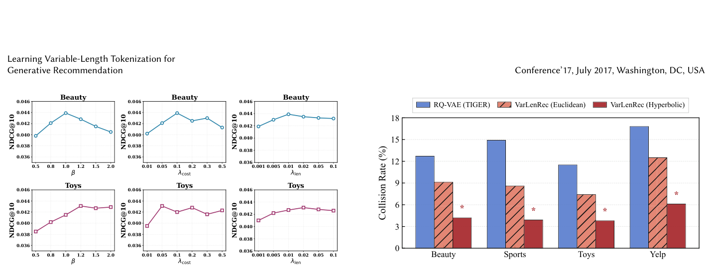
- $\beta$(PIBA 长度尖锐度):Beauty 在 $\beta=1.0$ 取得最佳,Toys 在 $\beta=1.2$ 取得最佳。$\beta$ 大则长度对 popularity 更敏感。
- $\lambda_{\text{cost}}$:Beauty $\lambda_{\text{cost}} = 0.1$、Toys $\lambda_{\text{cost}} = 0.05$ 最佳。太小则无 sparsity 正则,太大则过度惩罚。
- $\lambda_{\text{len}}$:Beauty $\lambda_{\text{len}} = 0.01$、Toys $\lambda_{\text{len}} = 0.02$ 最佳。太小则失去理论先验,太大则过度约束 gate 决策。
不同数据集最优配置不同——超参需要针对 catalog 特性调。
与已归档相关工作的对比¶
CapsID CapsID: Soft-Routed Variable-Length Semantic IDs for Generative Recommendation(2026-05-06)¶
关系:独立并发(本文未引用 CapsID,CapsID 也未引用本文,两者殊途同归)· 已加载对方精读
- 共同关注的问题:两篇都明确诊断"固定长度 SID 是 GR tokenizer 未审视的设计选择",并都用 stratified 实证证明易 / 难 item 需要不同 token 预算(CapsID 用 head/torso/tail R@10 + Proposition 2 上界;VarLenRec 用 Popularity-Length Paradox + Theorem 1 闭式解)。两者都同时识别"变长引入下游 collision + length-bias + hallucination"三难题并各自给出解。
- 相近的技术骨架:核心都是confidence/popularity 驱动的可微变长 controller——CapsID 用 capsule routing 的 max softmax weight × output norm 作为停止 confidence($q_{i,\ell} = \max_k c_{i,\ell k}^{(T)} \cdot \|\mathbf{o}_{i,\ell}^{(T)}\|$,$L_i = \min\{\ell: q_{i,\ell} \ge \tau \text{ or } \|\mathbf{r}_{i,\ell}\|_2 \le \epsilon \text{ or } \ell = L_{\max}\}$);VarLenRec 用 gate MLP 输出的 layer retention probability + cumulative mask($\alpha_i^{(l)} = \sigma(\mathrm{MLP}([\log_0^c \mathbf{r}; \log_0^c \mathbf{e}]))$,$m_i^{(l)} = \prod_j \alpha_i^{(j)}$,$L_i = \arg\max_l m_i^{(l)} \ge \tau$)。两者都用累积形式保证 prefix 约束。两者都加 length cost loss 抑制过长,都用辅助 codebook / disambiguation token 解碰撞、用 trie-constrained beam search 防 hallucination。
- 本文的差异与推进:
- 理论起点不同:CapsID 把长度决策放在"item-intrinsic 难度"上(残差范数 + 路由 confidence),VarLenRec 直接把长度与 statistical popularity 挂钩,给出闭式 $L_i^* = C \cdot p_i^{-\alpha/\gamma}$——本文先验更强,可解释性更好。CapsID 没有"长度 vs popularity"的解析公式。
- 几何空间不同:CapsID 仍在欧氏,靠 capsule routing 增加表达力;VarLenRec 引入Poincaré ball + Mobius algebra + Riemannian Adam,用 hyperbolic 指数体积承载差异化容量。VarLenRec 的 Euclidean 消融正是为了证明 hyperbolic 增益(Beauty R@10 -6.2%)。
-
监督路径:CapsID 的长度只由 confidence/residual 阈值"被动"触发;VarLenRec 的 PIBA 既提供长度先验也作为 length alignment loss $\mathcal{L}_{\text{len}}$ 的硬目标"主动"监督 gate——这是两者训练信号最显著的差异。
-
可比的方法 / 实验差异:两者都在 Amazon Beauty/Sports/Toys 上做主实验,但 CapsID 还有 35M item 工业目录(社交媒体平台),VarLenRec 多了 Yelp。CapsID 学到的平均长度 $\bar{L} \in [3.41, 3.89]$(hard cap $L_{\max} = 6$),VarLenRec 在 $L_{\max} = 10$ 下学到 $[5.31, 7.05]$(粒度更细,给 tail 更多空间)。Collision rate:CapsID 在三个公开集都 ~13%;VarLenRec 在 HARQ 下降到 ~3.2%,hyperbolic 几何的 collision 控制能力更强。两者结合(hyperbolic + capsule routing + popularity prior)很可能是下一个改进方向——两边各自的消融都暗示这些组件正交,未来工作值得在同一框架内同时实验。
讨论与局限性¶
核心贡献的工程价值¶
- PIBA 是把"变长直觉"转成工程实践的关键——其他方法(CapsID、ADA-SID)都隐式地用 confidence 阈值或 utilization 反推长度,VarLenRec 直接从信息论给出 $L^* \propto p^{-\alpha/\gamma}$,让长度可解释、可调、可验证。$\beta$ 超参直接控制 popularity sensitivity,部署时一目了然。
- Hyperbolic geometry 的几何动机非常清晰——附录 D 的三条定理(Hyperbolic Representational Capacity、Tree Embedding Distortion、Radial-Depth Correspondence)联合论证了"item 语义的树状结构 + 指数容量需求 → Poincaré ball 是几何上的自然选择"。Euclidean baseline 在 collision rate 与 R@10 上同时落后是直接证据。
- 效率反直觉地变好——一般变长机制会带来 overhead,VarLenRec 实际减少 19.3% 测试时间。原因是 popular item 用短 ID(这部分占 token 处理总量大多数),节省的 decoding step 覆盖了 hyperbolic 算子的额外开销。这点对工业部署很有吸引力。
局限与争议¶
- PIBA 假设 popularity 是长度的唯一驱动力——但语义复杂度(如多 facet item)独立于流行度也会增加 ID 长度需求。Length Prediction 消融(w/ Direct PIBA Assignment 比 full 低 3.0-7.0%)证明 content-aware soft gate 是必要的——纯 PIBA 不够,但论文没把"content complexity"显式建模成独立项。
- 冷启动 item 无 popularity——论文 §3.4 末讨论保守地分配 $L_{\max}$ 给冷启 item。这是合理但保守的选择,与 PIBA 的"信息论最优"哲学不完全自洽(冷启 item 信息缺口大但也可能内容简单)。
- Hyperbolic 算子的数值稳定性——附录 E 提到要做 safety margin $\epsilon = 10^{-5}$ 防止 codebook 飞出 ball,在 large-scale 训练时这种 boundary safeguard 是否会带来 silent degradation 没有定量分析。
- 没有工业 A/B——所有实验都是公开 benchmark,没有线上指标支撑(与 CapsID 的 35M 工业目录、AdaSID 的 Kuaishou 在线 A/B 形成对比)。论文末段讨论 enterprise deployment 是 forward-looking 而非已验证。
- 理论假设的近似性:Theorem 1 的推导需要 $\theta p_i \gg 1$ 才能用 $\log(1 + \theta p_i) \approx \log \theta + \log p_i$——但 tail item 的 $\theta p_i$ 恰恰是小的,正幂次衰减的近似在最需要它的 tail 区域反而最弱。论文未讨论这一近似的边界条件。
与已有工作的差异¶
- 与 TIGER / LETTER / ETEGRec / LC-Rec:这些都是 fixed-length tokenizer,VarLenRec 是首个 popularity-adaptive variable-length。
- 与 CapsID(独立并发):见上节专章——同问题、不同 root cause(popularity vs item-intrinsic 难度)、不同几何(hyperbolic vs euclidean)、不同监督(PIBA prior loss vs pure confidence 阈值)。
- 与 CRAB / CARD(codebook 偏置调控):这些方法在固定长度内做改进(CRAB 拆 popular token、CARD 做 uniform pre-warping);VarLenRec 直接换掉"固定长度"这条假设。两者正交,可以叠加。
- 与 QuaSID / AdaSID(碰撞处理):碰撞与长度是不同问题。VarLenRec 通过 hyperbolic + 变长本身就大幅降低碰撞(12.7% → 3.2%),不需要 QuaSID/AdaSID 的复杂 reweighting。
总结¶
VarLenRec 是 GR tokenizer 系列工作中第一篇把"长度本身"作为可学习量的工作,通过 PIBA 提供闭式 popularity-length 公式、HARQ 提供匹配几何容量、Soft Length Controller 提供可微优化通路、下游集成三件套保证检索可用性。最大的科学贡献是 Popularity-Length Paradox 的实证发现——这是一条所有 GR 后续工作都应该意识到的设计约束。CapsID(独立并发)从不同角度(capsule routing + content-confidence)回到了相同的"变长"结论,本身就是这条设计原则正确性的旁证。建议后续工作把 hyperbolic geometry、capsule routing、popularity prior 三者结合,并在工业系统中做 A/B 验证 length adaptation 对长期指标的影响(特别是冷启动与长尾流量分布的演化)。